Rodger's Sat Tracker

Engineering View Of A Standalone Satellite Tracker

Rodger's Sat Tracker

The app is approachable for any satellite user. This site presents the engineering layer underneath it: live SGP4 propagation, NORAD TLE refresh, Doppler correction, GPS-derived QTH, orbital ground tracks, and space-weather decision support.

Live Orbits SGP4 propagation in real time
Doppler Live RF shift correction as it happens
GPS QTH Location grid and locator tools
Space Weather Solar and geomagnetic alerts
Satellites Tracked
NORAD Refresh
Visible Passes Today
Space Weather

Orbital Dynamics Core

The website shows the technical layer that the everyday app hides.

Rodger's Sat Tracker tracks satellites from current NORAD two-line elements through SGP4, then converts the propagated state into the operator quantities that matter during a pass: subpoint, altitude, footprint, slant range, elevation, azimuth, and live RF Doppler.

01

SGP4 State Propagation

Live CelesTrak TLEs create the satellite record, then SGP4 propagates the ECI state for the selected NORAD object. That position becomes the source for every map, pass, and RF calculation. It also keeps every visible label tied to the current epoch and selected satellite.

\[ \mathbf r_{\mathrm{ECI}}(t)= \mathrm{SGP4}\!\left(\mathrm{TLE},JD,fr\right) \]
02

Observer Elevation

Observer latitude, longitude, altitude, and satellite range resolve into local azimuth and elevation. The interface uses that geometry to mark above-horizon tracks, pass windows, and pointing decisions. That station frame keeps pass visibility and antenna motion physically grounded.

\[ El = \operatorname{atan2}\!\left( \rho_U,\sqrt{\rho_E^2+\rho_N^2} \right) \]
03

Doppler Correction

Relative range-rate from the propagated pass becomes a live Doppler estimate for receive and transmit planning. The RF pane keeps frequency offset tied to the current spacecraft geometry. This prevents tuning decisions from drifting away from the pass geometry.

\[ \Delta f \approx -f_0\frac{v_r}{c} \]
04

Earth Footprint

Orbital altitude determines the visibility cone and footprint radius on Earth. The map turns that geometry into a practical coverage, acquisition, and station-in-range decision tool. Operators can quickly see whether the ground site sits inside the usable pass footprint.

\[ \theta_f = \cos^{-1}\!\left(\frac{R_E}{R_E+h}\right) \]

Operations Console

A simple user experience backed by orbital, RF, and ionospheric context.

The application combines pass prediction, live telemetry, antenna pointing, Doppler, local QTH, solar flux, Kp index, X-ray flux, HF band state, DX cluster, and AMSAT news in the same workflow. This page exposes those engineering relationships for a technical audience.

Rodger's Sat Tracker 3D globe view with satellite labels, orbit tracks, sun marker, and GPU status.

3D Globe + 2D Map

Switch between a textured Earth globe and a ground-track map with footprints, day/night shading, trails, and selected satellite labels.

Pass Timeline

AOS, LOS, maximum elevation, current state, and countdowns are surfaced where an operator can act on them quickly.

GPS Lock + Maidenhead

GPS/manual QTH feeds latitude, longitude, altitude, and grid square calculations for accurate local tracking geometry.

Application Screens

Every screen has an engineering job.

These are actual Rodger's Sat Tracker application views. Each one is tied to the calculation, signal decision, or orbital-control problem it helps an operator solve.

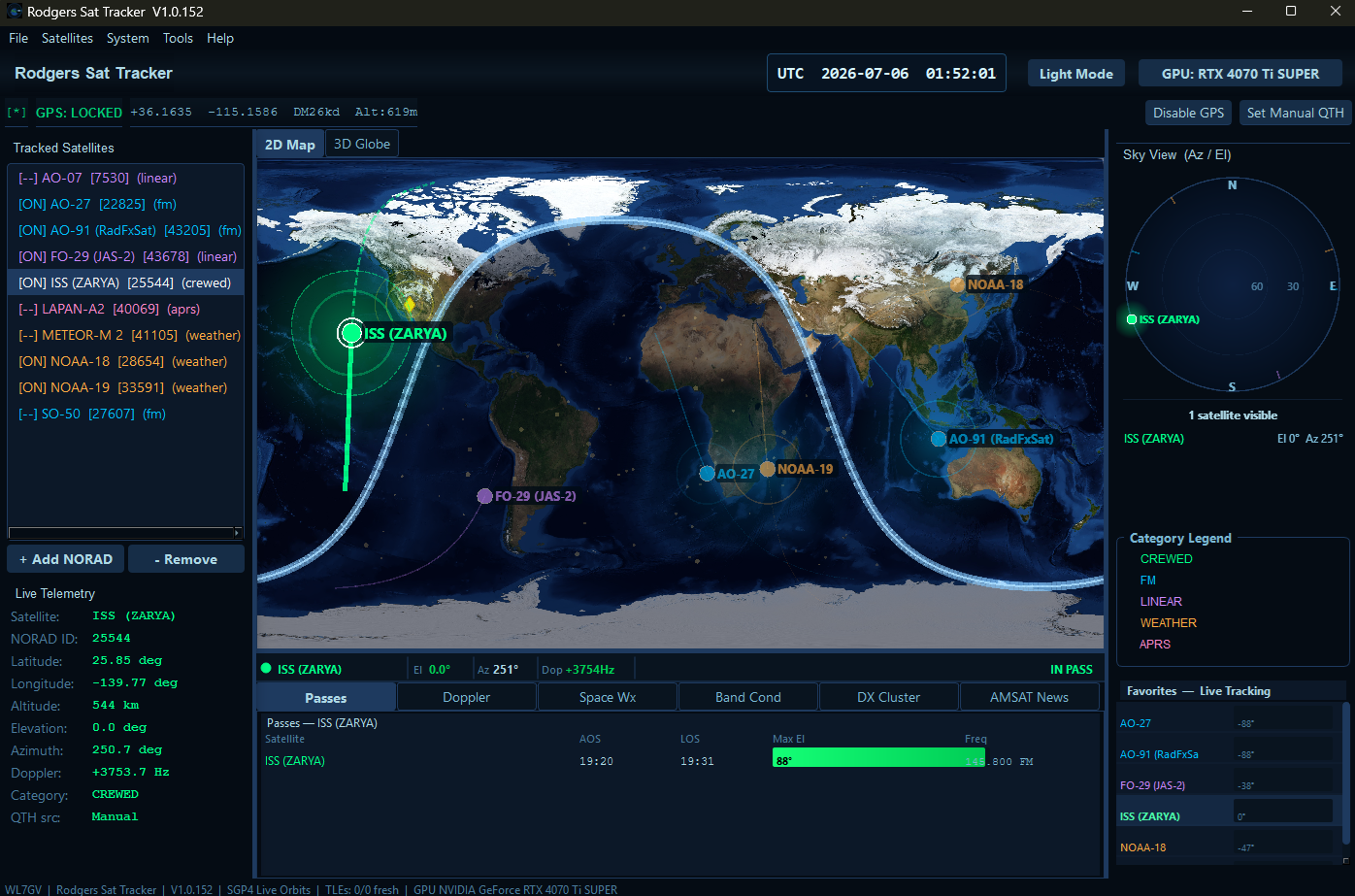
2D ground track map with satellite footprint, telemetry, pass prediction, and sky view.
Bottom readout: Rodger's Sat Tracker | SGP4 Live Orbits | TLEs fresh | GPU NVIDIA GeForce RTX 4070 Ti SUPER
2D computation stack SGP4 state -> subpoint -> footprint -> pass table -> Doppler state -> sky view

The screen combines the propagated orbit, observer geometry, and RF state so the operator does not have to cross-check separate tools during a live pass.

2D Map / Ground Track / Footprint

Turns propagated orbital state into a usable pass map.

The 2D map is where Rodger's Sat Tracker makes the SGP4 state visible: current subpoint, future path, footprint rings, day/night context, pass table, Doppler status, and sky-view pointing all sit in one operator frame.

  • Input: TLE epoch, observer QTH, current UTC, and selected NORAD catalog object.
  • Output: latitude, longitude, elevation, footprint radius, pass state, and Doppler-ready range-rate.
  • Operator value: the same frame answers where it is, where it is going, and whether it is usable now.
\[ \mathbf r_{\mathrm{ECI}}(t),\mathbf v_{\mathrm{ECI}}(t) = \mathrm{SGP4}\!\left(\mathrm{TLE},t\right) \] \[ \lambda = \operatorname{atan2}(y,x)-\theta_{\mathrm{GMST}}, \qquad \phi = \tan^{-1}\!\left(\frac{z}{\sqrt{x^2+y^2}}\right) \] \[ \theta_f = \cos^{-1}\!\left(\frac{R_E}{R_E+h}\right) \]

Why it matters: the operator can see where the spacecraft is, where it is going, whether the ground station is inside the visibility footprint, and whether the pass is actionable right now. The map also keeps pass timing, footprint geometry, sky-view pointing, and Doppler state tied to the same propagated object instead of forcing separate cross-checks.

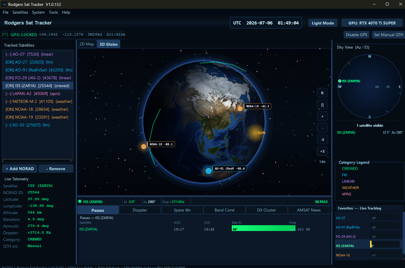
Rodger's Sat Tracker 3D globe view with satellite labels, orbit tracks, sun marker, and GPU status.
Bottom readout: W7GV | Rodger's Sat Tracker | SGP4 Live Orbits | TLE freshness | GPU acceleration
3D frame stack ECI vector -> Earth rotation -> ECEF scene -> orbit arc -> sun marker

The globe view makes frame rotation, orbital plane, illumination, and moving subpoint geometry visible at the same time. It keeps Earth-fixed context, orbit arc direction, and sun geometry in one spatial readout.

3D Globe / Earth Frame / Sun Marker

Shows orbit geometry as a real spatial relationship.

The 3D globe view makes inclination, orbital plane, subpoint motion, Earth rotation, and sunlight geometry easier to understand than a flat map alone. It is especially useful for explaining why the same spacecraft can appear rapidly changing in azimuth and elevation during a LEO pass.

  • Frame logic: inertial state vectors are rotated into the Earth-fixed frame for display.
  • Lighting context: the sun marker and terminator help separate visibility geometry from illumination.
  • Engineering use: orbit plane, inclination, and subpoint motion become inspectable instead of abstract.
\[ \mathbf r_{\mathrm{ECEF}} = R_3\!\left(\theta_{\mathrm{GMST}}\right)\mathbf r_{\mathrm{ECI}} \] \[ \delta_\odot = \sin^{-1}\!\left(\sin \varepsilon \sin \lambda_\odot\right), \qquad \lambda_\odot \approx -15^\circ\left(UT-12\right) \]

Why it matters: the 3D view gives engineers an immediate mental model of orbit plane, Earth-fixed projection, lighting, and relative motion. It also shows why ground-track motion and sky-view motion can change quickly during the same LEO pass. That makes the display useful for explaining why a satellite can look smooth on the map while sweeping rapidly across the local sky. The same view helps compare orbit arc, Earth rotation, illumination, sun marker placement, and moving subpoint geometry in one operator-readable frame.

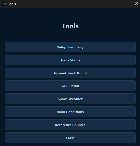
Tools dialog listing setup summary, track status, ground track detail, GPS detail, space weather, band conditions, and reference sources.
Dialog readout: Setup Summary / Track Status / Ground Track Detail / GPS Detail / Space Weather / Band Conditions / Reference Sources

Tools / Mission Workflow

Separates the operator workflow into decision surfaces.

The tools menu is not filler. It is a structured entry point into setup, tracking, ground track detail, station reference, propagation weather, band condition, and source-reference views.

  • Workflow: setup and status screens keep inputs separate from live tracking outputs.
  • Auditability: GPS, TLE, propagation, RF, and reference-source decisions can be checked independently.
  • Traceability: each tool maps to a specific setup, tracking, propagation, RF, band, or reference decision.
\[ \mathcal O = \{\mathrm{setup},\mathrm{status},\mathrm{track},\mathrm{QTH}, \mathrm{space\ weather},\mathrm{bands},\mathrm{refs}\} \] \[ \mathrm{Decision}(t) = f\!\left(\mathrm{TLE},\mathrm{QTH},\mathrm{El}(t),\Delta f(t),K_p,SFI\right) \]

Why it matters: engineers can audit each input to the final contact decision instead of treating the tracker as a single opaque display. The tools menu keeps setup, station geometry, propagation weather, RF planning, and reference checks separated enough to verify before a live pass.

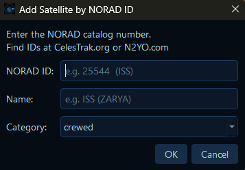
Add Satellite by NORAD ID dialog with category selection.
Input readout: NORAD ID + satellite category creates the catalog binding used for TLE lookup and mode context.
Catalog binding path NORAD 25544 -> TLE lines -> SGP4 satellite record -> UI object

The dialog creates the identity link that keeps every later map, pass, Doppler, and mode calculation attached to the correct spacecraft. The NORAD ID selects the TLE source, the name keeps the operator label readable, and the category preserves RF context for the rest of the workflow.

Validated operator input catalog ID -> satellite name -> category -> tracking mode

This prevents a visual label, RF mode, pass table, and propagated state from drifting into separate meanings. One clean catalog binding becomes the shared key for map labels, Doppler calculations, sky-view pointing, and operator notes.

NORAD ID / TLE Binding

Catalog identity is the key that connects the UI to orbital data.

Adding a satellite by NORAD catalog number lets Rodger's Sat Tracker bind a human-readable satellite entry to the two-line element set used by SGP4. The category also drives RF and operator context such as crewed, FM, linear, weather, and APRS tracking modes, so the selected object carries both orbital state and mission meaning.

  • Identity: the catalog number prevents confusing one spacecraft state vector with another.
  • Mode metadata: category tags support operator decisions beyond raw orbital position.
  • TLE binding: the selected ID resolves to the line pair that initializes the SGP4 satellite record.
  • Workflow continuity: the same identity drives labels, pass tables, Doppler state, and screen context.
\[ n_{\mathrm{NORAD}} \rightarrow \left(L_1(n),L_2(n)\right) \rightarrow \mathrm{Satrec}(n) \] \[ \mathbf x_n(t)= \left[\mathbf r_n(t),\mathbf v_n(t)\right] = \mathrm{SGP4}\!\left(L_1(n),L_2(n),t\right) \]

Why it matters: the catalog number is what keeps pass prediction, map labeling, Doppler, and satellite-specific workflow tied to the correct object. Without that binding, an operator could trust a clean-looking track while using the wrong spacecraft identity, RF category, or TLE epoch.

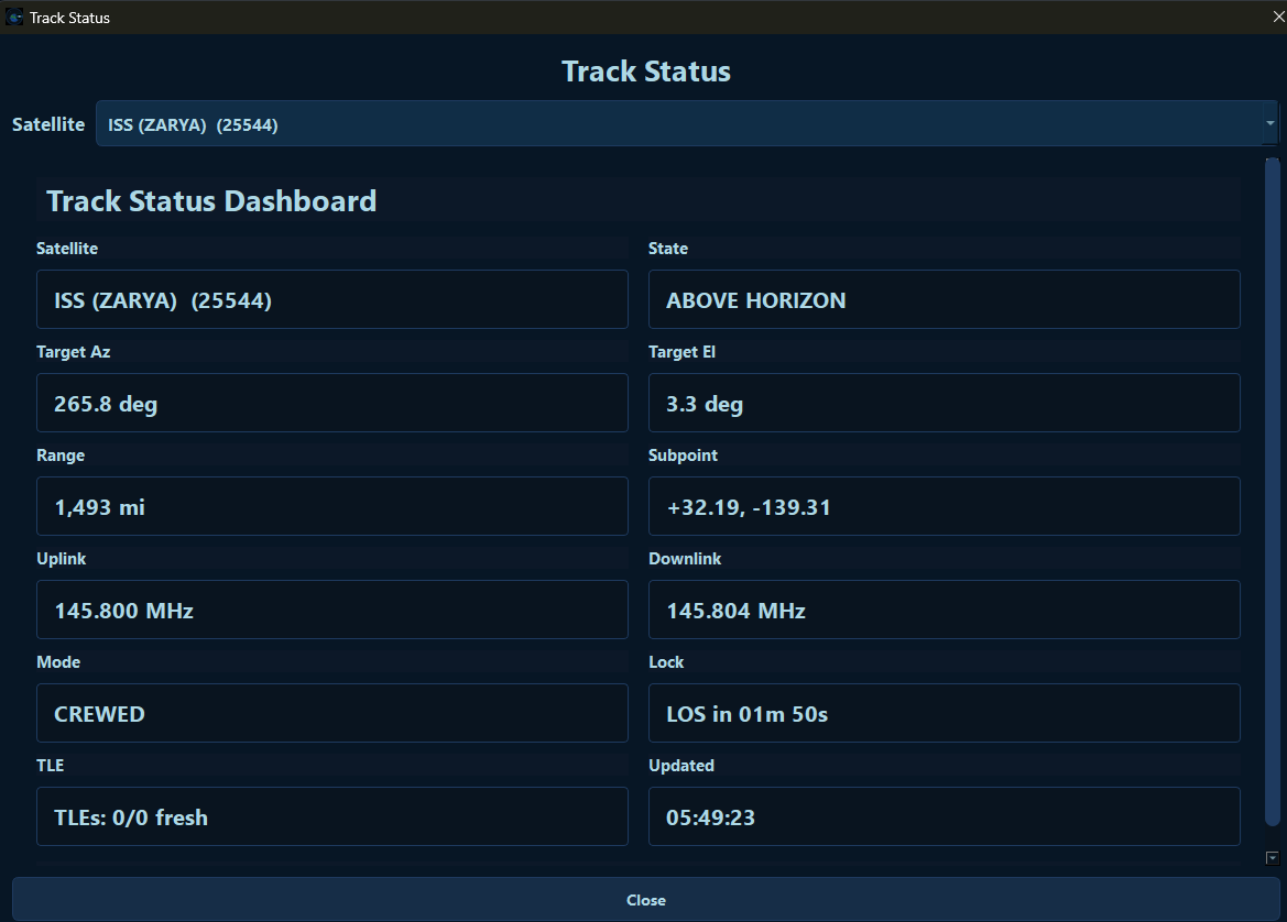
Track Status dashboard with satellite state, azimuth, elevation, range, uplink, downlink, mode, and lock time.
Status readout: azimuth, elevation, range, subpoint, uplink, downlink, mode, Doppler, and AOS/LOS timing.
Live action values azimuth / elevation / range / Doppler / AOS / LOS / mode

This is the operator-facing reduction of the full orbital solve: where to point, what frequency offset to expect, and how much pass time remains.

Track Status / Az-El / Range / Doppler

Reduces orbital motion to antenna and radio actions.

This dashboard translates propagated position into the numbers an operator needs while the pass is happening: azimuth, elevation, range, subpoint, uplink/downlink frequency, mode, and time to LOS or AOS.

  • Antenna solve: topocentric east-north-up projection becomes azimuth and elevation.
  • RF solve: range-rate becomes a Doppler correction rather than a visual guess.
  • Timing solve: AOS and LOS state give the operator a pass clock.
\[ \boldsymbol\rho = \mathbf r_{\mathrm{sat}}-\mathbf r_{\mathrm{obs}}, \qquad \rho = \lVert \boldsymbol\rho \rVert \] \[ El = \sin^{-1}\!\left( \frac{\boldsymbol\rho\cdot\hat{\mathbf u}}{\lVert\boldsymbol\rho\rVert} \right), \qquad Az = \operatorname{atan2}\!\left( \boldsymbol\rho\cdot\hat{\mathbf e}, \boldsymbol\rho\cdot\hat{\mathbf n} \right) \] \[ \Delta f \approx -f_0\frac{v_r}{c} \]

Why it matters: LEO passes move fast. If azimuth, elevation, and Doppler are not presented together, the operator is forced to stitch together time-critical decisions manually.

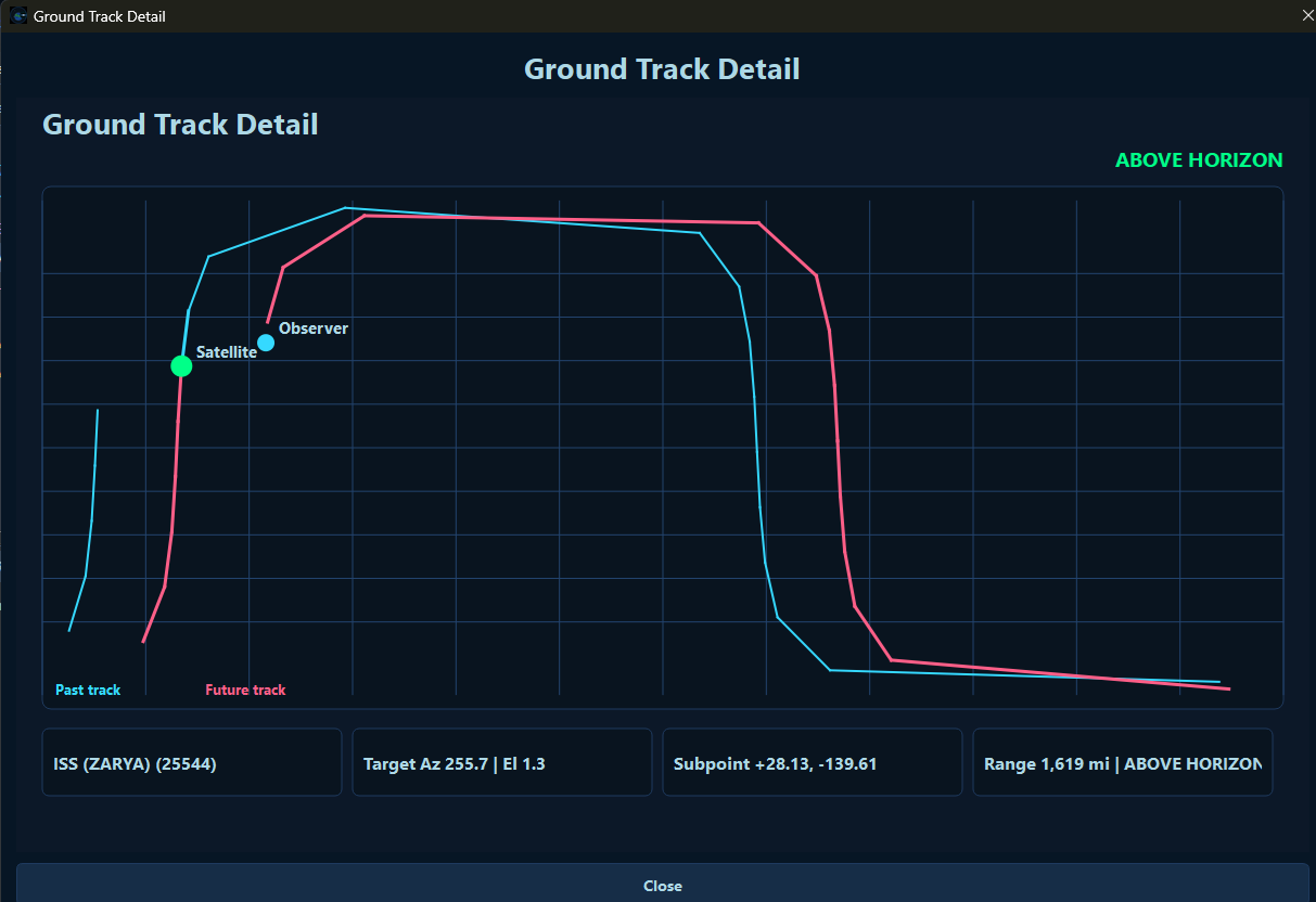
Ground track detail display showing past and future orbit traces, observer point, satellite point, and above-horizon state.
Ground-track readout: ISS (ZARYA) 25544 | Target Az 255.7 | El 1.3 | Subpoint +28.13, -139.61 | Range 1,619 mi | ABOVE HORIZON
Track sampling window past samples + current state + future samples + horizon crossing

The graph is a time-indexed orbit trace, not a static picture. It shows how the pass approaches, peaks, and exits the station footprint.

Ground Track Detail / Past-Future Sampling

Samples the orbit around now so the operator can anticipate motion.

Rodger's Sat Tracker samples the selected satellite backward and forward in time around the current instant. The result is a past track and future track that explain where the satellite came from, where it is going, and when it crosses the local horizon.

  • Past path: recent samples explain the direction and curvature of the pass.
  • Future path: forward samples expose horizon crossing, peak geometry, and upcoming azimuth sweep.
  • Event logic: AOS and LOS are zero-elevation roots with opposite elevation-rate signs.
\[ \mathcal T = \left\{ \left(t_i,\phi_i,\lambda_i\right) \mid t_i=t_0+i\Delta t \right\} \] \[ \mathrm{AOS}: El(t)=0,\ \frac{dEl}{dt}>0 \qquad \mathrm{LOS}: El(t)=0,\ \frac{dEl}{dt}<0 \] \[ d = 2R_E\sin^{-1}\!\sqrt{ \sin^2\frac{\Delta\phi}{2}+ \cos\phi_1\cos\phi_2\sin^2\frac{\Delta\lambda}{2}} \]

Why it matters: the operator sees whether the pass is rising, peaking, or falling, and can understand the sky movement before it becomes urgent.

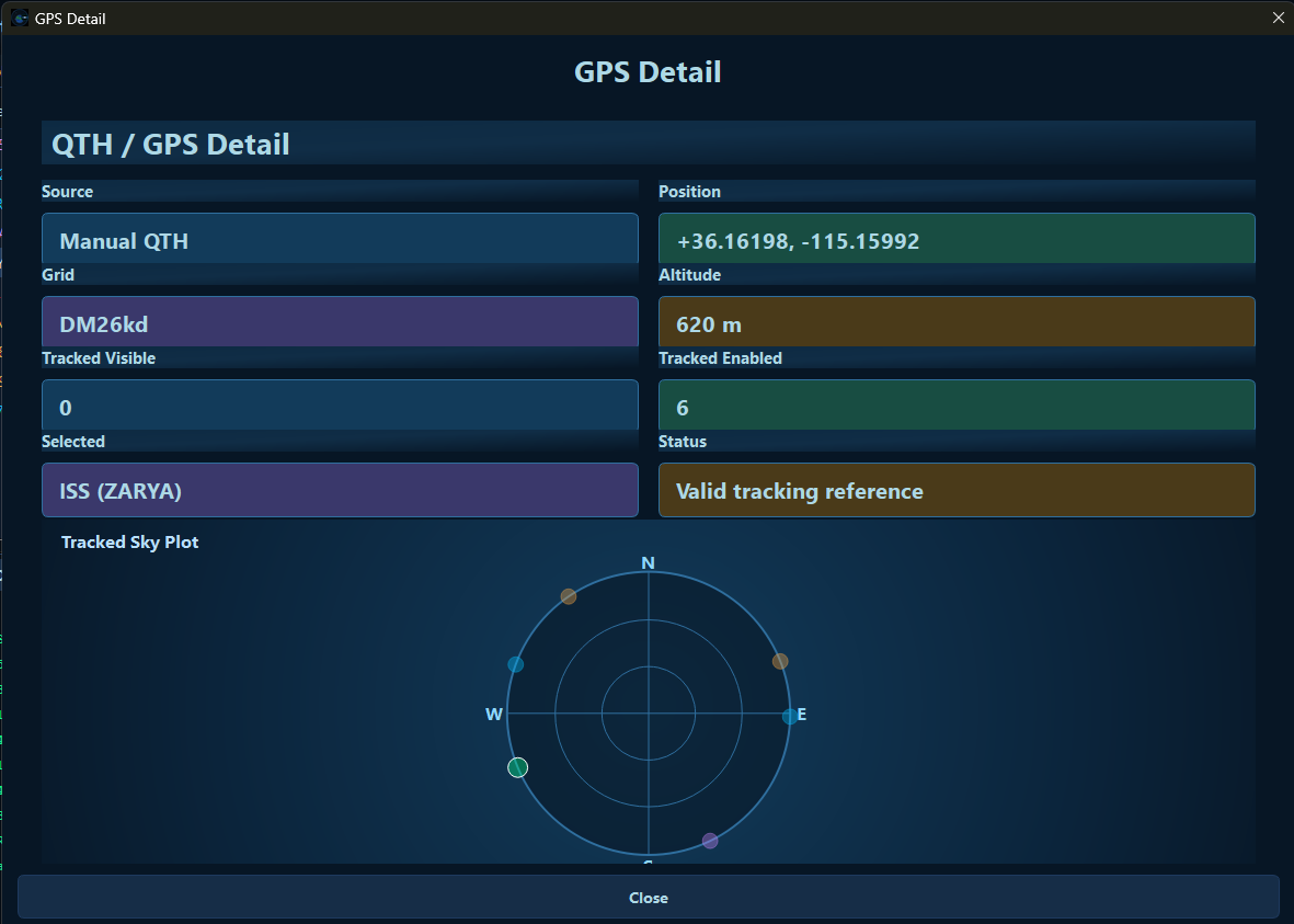
GPS detail panel showing QTH source, Maidenhead grid, position, altitude, enabled satellites, and tracked sky plot.
QTH readout: source, latitude, longitude, altitude, Maidenhead grid, enabled satellite count, and sky-view reference.
Observer reference frame GPS/manual QTH -> lat/lon/alt -> ENU basis -> Maidenhead grid

Every pass calculation is local to the observer. This screen exposes the station frame before azimuth, elevation, range, and Doppler are trusted.

GPS Detail / QTH / Maidenhead Grid

Locks the observer reference frame before solving the pass.

All azimuth, elevation, range, and Doppler values depend on the observer position. The GPS/QTH screen makes that input explicit: source, latitude, longitude, altitude, grid square, enabled satellite count, and sky plot.

  • Observer vector: latitude, longitude, and altitude define the local tangent plane.
  • Grid square: Maidenhead output supports amateur-radio logging, exchange, and planning.
  • Error path: bad QTH data propagates directly into pointing, timing, and range estimates.
\[ \mathbf r_{\mathrm{obs}} = \begin{bmatrix} (R_E+h)\cos\phi\cos\lambda\\ (R_E+h)\cos\phi\sin\lambda\\ (R_E+h)\sin\phi \end{bmatrix} \] \[ \mathrm{Grid}_{\mathrm{Maidenhead}} = g\!\left(\lambda+180^\circ,\phi+90^\circ\right) \]

Why it matters: a small QTH error becomes a real antenna-pointing and timing error during low-elevation passes.

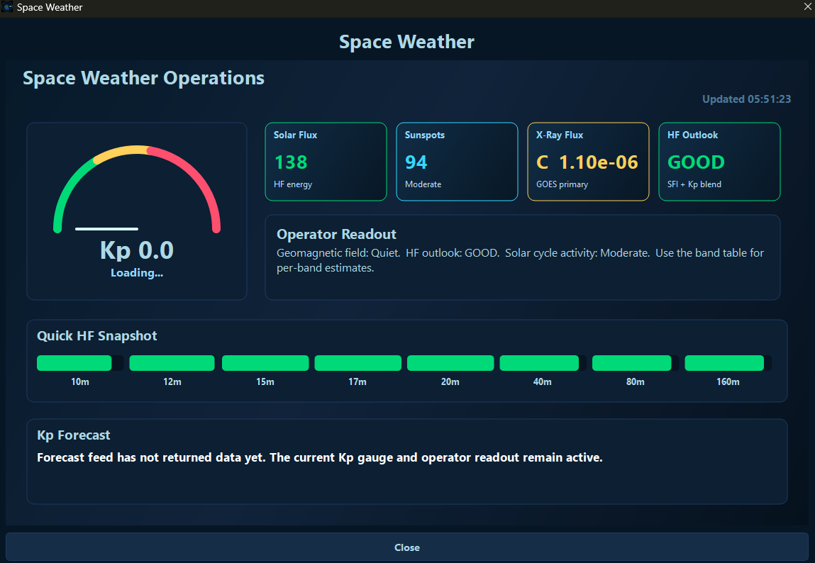
Space weather operations panel showing Kp, solar flux, sunspots, X-ray flux, HF outlook, and quick band snapshot.
Space-weather readout: Kp, solar flux index, sunspot number, X-ray class, HF outlook, and quick band snapshot.
Propagation environment Kp / SFI / SSN / X-ray class / HF outlook / band snapshot

The app keeps space-weather context near the pass data so failed contacts can be diagnosed as geometry, RF setup, or propagation conditions.

Space Weather / Kp / Solar Flux / X-Ray Flux

Adds ionospheric context to the satellite operations picture.

The space weather screen gives operators solar flux, sunspot count, Kp, X-ray class, and HF outlook in the same workstation. It helps explain whether link conditions are being shaped by the satellite pass or by the propagation environment.

  • Kp: geomagnetic disturbance context for auroral absorption and unstable propagation.
  • SFI and SSN: solar activity proxies used to reason about ionospheric support.
  • X-ray flux: flare context for shortwave fadeout and sudden ionospheric changes.
\[ K_p \uparrow \Rightarrow \mathrm{geomagnetic\ disturbance}\uparrow \] \[ f_{oF2} \approx 9\sqrt{N_{\max}}, \qquad \mathrm{MUF} \approx \frac{f_{oF2}}{\cos\chi} \] \[ \mathrm{Risk}_{HF} = F(K_p,\mathrm{SFI},X_{\mathrm{ray}},\mathrm{SSN}) \]

Why it matters: when a contact fails, the operator needs to separate geometry, station setup, and propagation conditions instead of guessing.

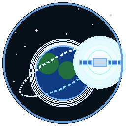
Band conditions panel showing HF bands with percentage quality bars and solar flux index.
Band readout: per-band quality bars, percentage-style score, solar-flux threshold state, and GOOD/FAIR/POOR labels.
Band scoring model SFI thresholding -> band percentage -> GOOD / FAIR / POOR decision

The bars turn solar-flux thresholds into a quick planning layer while the formulas show the scoring logic behind the visual result.

Band Conditions / SFI Scoring

Converts solar flux into a readable per-band operating estimate.

Rodger's Sat Tracker uses observed solar flux and band-specific thresholds to label bands as POOR, FAIR, or GOOD with a percentage-style readout. The exact score is intentionally operator-facing: it compresses propagation context into something usable during planning.

  • Thresholds: each HF band can use different fair and good solar-flux breakpoints.
  • Readable output: a visual bar compresses the propagation estimate without hiding the scoring logic.
  • Planning value: the band panel separates satellite geometry from terrestrial HF propagation context.
\[ p_b = \begin{cases} \min(100,\ 60 + 40\frac{SFI-G_b}{M_b-G_b}) & SFI \ge G_b\\ 25 + 35\frac{SFI-F_b}{G_b-F_b} & F_b \le SFI < G_b\\ \max(2,\ 25\frac{SFI}{F_b}) & SFI < F_b \end{cases} \] \[ C_b = \begin{cases} \mathrm{GOOD} & SFI \ge G_b\\ \mathrm{FAIR} & F_b \le SFI < G_b\\ \mathrm{POOR} & SFI < F_b \end{cases} \]

Why it matters: engineers can see the threshold logic behind the visual bars instead of reading a black-box propagation label.

Why The Features Matter

The app turns orbital mechanics into operator decisions.

TLE Ingest CelesTrak / NORAD IDs

Fresh two-line elements keep the state vector aligned with the catalog.

Propagation SGP4 + ECI/Earth mapping

The predicted orbit becomes latitude, longitude, altitude, ground track, and orbital trail.

Observer Solve QTH, Az, El, Range

Station coordinates determine whether the satellite is usable and where antennas must point.

RF Action Doppler + Pass Windows

Frequency offset and AOS/LOS timing keep the operator synchronized with fast-moving LEO passes.

Engineering References

The site should point engineers toward the same ecosystem the tracker depends on.

Rodger's Sat Tracker sits at the intersection of orbital mechanics, amateur satellite operations, RF Doppler correction, ground-station practice, and space-weather interpretation. These links and books are included as engineering context, not decorative filler.

Orbital Mechanics David A. Vallado, Fundamentals of Astrodynamics and Applications

Best fit for SGP4, ECI/ECEF transforms, perturbation thinking, and practical implementation details.

Classical Astrodynamics Bate, Mueller, and White, Fundamentals of Astrodynamics

Strong background for conics, two-body motion, state vectors, orbital elements, and time-of-flight reasoning.

Mission Design Wertz, Everett, and Puschell, Space Mission Engineering

Useful systems context for why tracking, ground station geometry, communications, and operations constraints matter together.

Amateur Satellite Operations ARRL and AMSAT satellite operating guides

Practical bridge between the equations, antennas, radios, Doppler correction, FM/linear satellites, and real operator workflow.

Accessible App / Technical Website

Local satellite tracking with the engineering layer exposed.

Rodger's Sat Tracker is a standalone Windows application for practical satellite work. The app stays approachable for everyday operators, while this website explains the technical layer behind each operator decision.

  • Orbit source: current NORAD two-line element sets are refreshed and bound to the selected spacecraft catalog identity.
  • Propagation: SGP4 produces time-tagged ECI position and velocity, then the interface converts that state into map, sky-view, pass, and RF quantities.
  • Station context: GPS or manual QTH provides latitude, longitude, altitude, and grid-square inputs for local azimuth, elevation, range, and Doppler solves.
  • Operator value: pass timing, footprint, Doppler, space weather, HF bands, DX cluster context, and AMSAT references stay in one workflow.
  • Engineering audit: each visible value can be traced back to orbit source, station location, UTC time, frame conversion, range geometry, and RF assumption.
  • Standalone reliability: the local Windows workflow keeps prediction, visualization, radio planning, and reference checks available without a cloud subscription.
Capability stack
Orbit Engine

Refreshed NORAD TLEs stay tied to the selected catalog identity while SGP4 propagates the spacecraft state forward in UTC. The interface turns that state into position, velocity, ground track, subpoint, altitude, and coverage footprint geometry. That same state drives visibility, timing, map labels, and pass decisions.

Live Pass View

The 2D map, 3D globe, sky-view pointing, AOS/LOS timing, visible-pass state, and pass tables stay in one operator frame so antenna direction, pass timing, and spacecraft motion remain readable together. Engineers can check current visibility, future motion, and operator action without leaving the tracking view.

RF Chain

Range-rate is translated into live Doppler correction for receive and transmit planning. FM, linear, weather, APRS, and crewed categories preserve operating context beyond raw orbital position. Tuning decisions stay tied to pass geometry, elevation, and mode category as range changes through the contact.

Decision Support

GPS QTH, Maidenhead grid, space weather, HF band conditions, DX cluster context, AMSAT news, and reference sources keep propagation and operating decisions close to the pass workflow. The operator can see whether a pass issue is orbital, station-location, radio, or propagation related.